Fast Random Projections in CUDA
[August 15, 2024]
Random projections are a powerful tool for dimensionality reduction. Specifically, if we start with $b$ points in $\mathbb{R}^D$, we can left-multiply all of them by a random matrix $R \in \mathbb{R}^{k \times D}$ (where $k \ll D$). We then end up with $b$ points in $\mathbb{R}^k$. It turns out that these projected points nearly preserve the distance relations of the original points.
Due to this property, random projections are very useful in statistics and machine learning problems dealing with high-dimensional data.
In this writeup, I won’t focus on the uses of random projections, but rather on how to efficiently implement them in CUDA. Specifically, I think that random projections nicely showcase both the benefits and challenges of exploiting sparsity on GPUs.
Problem Setup
Let’s first define the problem. We want to compute a product $Y = RA$ where:
- $R \in \mathbb{R}^{k \times D}$ is a random matrix. Each entry is uniformly randomly selected to be either -1 or 1
- $A \in \mathbb{R}^{D \times b}$ is a matrix storing a batch of $b$ $D$-vectors. The batch dimension $b$ is typically quite small (~32) while $D$ is enormous (can be hundreds of millions)
- $Y \in \mathbb{R}^{k \times b}$ is the product matrix.
The nice thing about random matrices is that you don’t need to store them. Instead, we can generate entries of $R$ on the fly and immediately multiply them with the appropriate entries of $A$. If we want to multiply with the same $R$ matrix multiple times, we just need to use the GPU’s pseudorandom generator seeding. Prior work has done this and it works great.
Computing $Y = RA$ this way takes $k \cdot D \cdot b$ multiplications.
An Algorithmic Improvement
It would be cool if we could achieve the same result with less computation (and therefore get speedups). A 2006 paper “Very Sparse Random Projections” provides us a neat way of achieving this goal. Instead of generating (and multiplying by) by $R$, we can achieve statistically equivalent results by multiplying with a much sparser matrix $S$, defined in terms of a parameter $p$ (the probability that any entry is nonzero):
\[S_{i,j} = \begin{cases} 1 & \text{with probability } \frac{p}{2}, \\-1 & \text{with probability } \frac{p}{2}, \\0 & \text{with probability } 1 - p.\end{cases}\]The resulting matrix only has $p$ times as many nonzeros as the original dense $R$ matrix. In the paper, they shows that constructing $S$ with $p = \frac{1}{\sqrt{D}}$ will still be good at preserving distances. Given the fact that we don’t actually need to evaluate multiplications by 0, for $D$ = 100,000,000 this is a 10,000x reduction in work!
Computing $Y = RA$ using this trick only takes $k \cdot \sqrt{D} \cdot b$ multiplications.
General Approach
While this huge work reduction is fantastic, we still need to figure out how to make it work in practice. For concreteness, let’s look at a small example with $b = 4, D = 16, k = 5$:
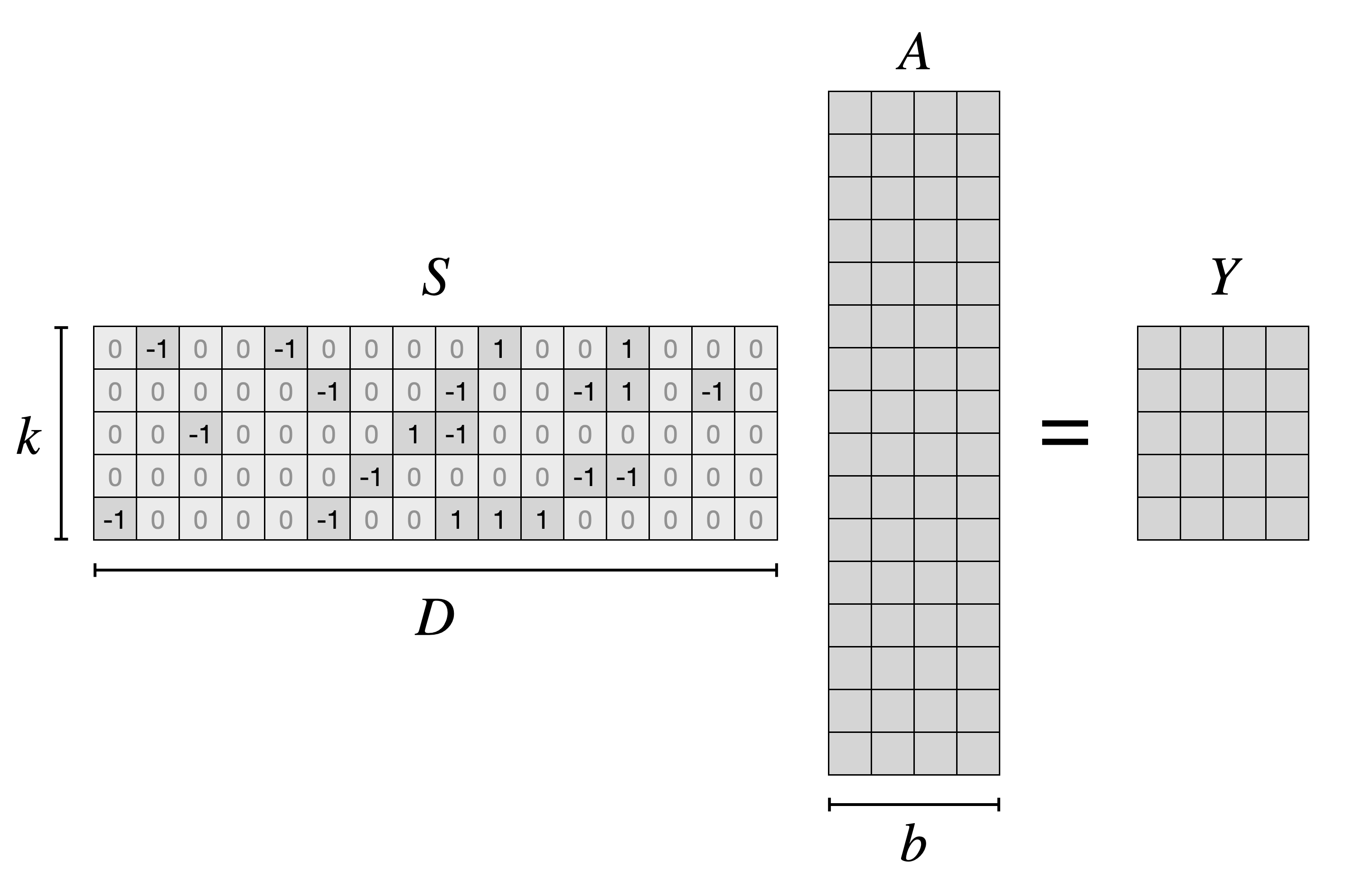
Our $S$ matrix is sparse: only a $\frac{1}{\sqrt{D}} = \frac{1}{4}$ fraction of entries are nonzero. We could just generate the $S$ matrix entirely, multiply it by the $A$ matrix using the GPU’s fast matrix-multiply units and be done with it… but then the sparsity would provide no advantage at all!
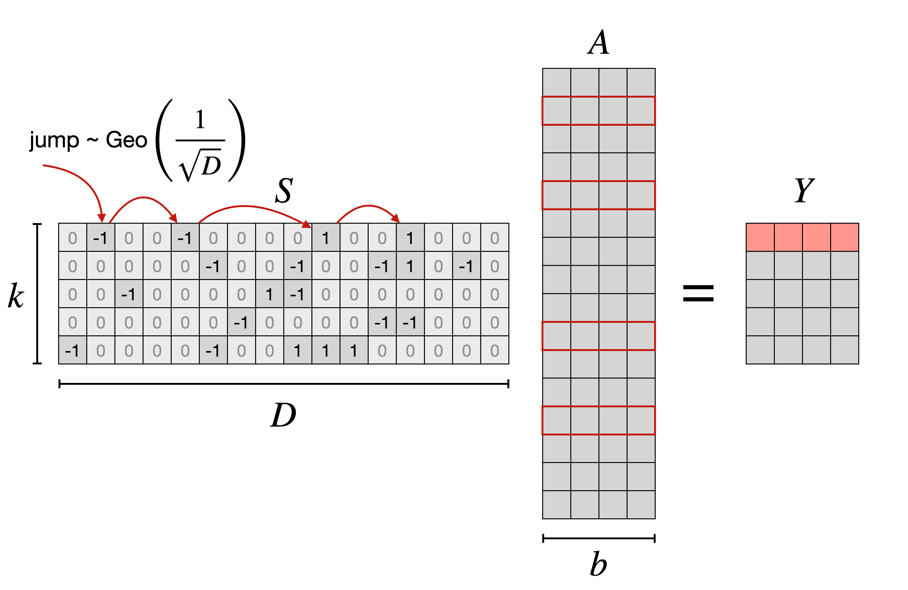
Instead, let’s use a trick from probability. Suppose we walk along the top row of the matrix flipping a coin that comes up heads $\frac{1}{\sqrt{D}}$ of the time. When it comes up heads, we drop a nonzero where we’re standing (50/50 whether it’s a 1 or -1). The distance we walk between placing nonzeros will be geometrically distributed with rate $\frac{1}{\sqrt{D}}$. This gives us an algorithm for multiplying a row $S_i$ by the $A$ matrix and producing a row $Y_i$:
idx = 0
while idx < D:
    jump = np.random.geometric(1 / np.sqrt(D))
    idx += jump

    sign = -1 if np.random.random() < 0.5 else 1
    Y[i] += A[idx,:] * sign
Here’s a visual depiction of the algorithm:
CUDA Implementation v1
A natural first attempt might look like this. A GPU has many threads, we assign each thread to a row of $S$, then have the thread execute the algorithm shown above.
__global__ void kernel_v1(TorchMatrix input, TorchMatrix output,
            uint32_t D, uint32_t k, uint32_t seed, float p) {

    float lambda_inv = 1.0 / p;
    uint32_t row = blockIdx.x * blockDim.x + threadIdx.x;

    curandStateXORWOW_t random_state;
    curand_init(seed, row, 0, &random_state);

    uint32_t idx = 0;
    while (true) {
        float u = curand_uniform(&random_state);
        uint32_t jump = (uint32_t) ((-logf(u)) * lambda_inv);

        bool sign = curand_uniform(&random_state) > 0.5;
        float coeff = sign ? 1.0 : -1.0;

        idx += jump;
        if (idx >= D) {
            break;
        }

        for (uint32_t i = 0; i < batch_size; i++) {
            output[row][i] += coeff * input[idx][i];
        }
    }
}
This approach works decently well. On an Nvidia A100, with $b = 32, k = 16,384, D = 10,000,000$, the dense baseline implementation ran in ~1.3 seconds. When $S$ has a density $\frac{1}{\sqrt{D}} = \frac{1}{10,000}$, this kernel runs in only 215 milliseconds… a 6$\times$ speedup!
However, it is doing ~10,000$\times$ fewer multiplications. All of a sudden, 6$\times$ doesn’t feel so good. This is an example of the sparsity tax. While we are doing a lot less work, modern GPUs are much more efficient at dense computations. So, much of what we gain by doing less work, we give back via less hardware-friendly code.
By optimizing the code and making it more GPU friendly, we can pay less sparsity tax.
CUDA Implementation v2
Implementation v1 assumes that all GPU threads are totally independent instruction streams, just like pthreads on a CPU. This is wrong and costs a lot of performance.
In fact, “threads” on a GPU are actually just one of a vector processor’s lanes. Every group of 32 threads (a “warp” in Nvidia terminology) executes in lockstep. This has major performance implications. For example, suppose that on the first while loop iteration, thread 0 (responsible for row 0) randomly draws a jump of 373 and thread 1 draws a jump of 1123. When these threads get to the first iteration of the inner loop (output[row][0] += coeff * input[idx][0]), thread 0 will have idx = 373 and thread 1 will have idx = 1123. When they both try to load input[idx][0] (because they are just lanes in the same warp, this will be issued as a single vector load instruction), this instruction will need to find data at multiple completely different memory locations: input[373] and input[1123]. In reality, because there are 32 threads in a warp, it would also need to find data at 30 other random memory locations too!
Performancewise, this is extremely painful. One load instruction results in 32 serialized data transfers. In Nvidia terminology, a single load instruction needing to find data in non-adjacent locations is called an “uncoalesced load”. Let’s try to fix this.
Instead, we can do the following:
- assign each warp to a row of $S$. We only calculate one
jumpat a time per warp. - assign each lane (thread) within the warp to a column of $A$, effectively parallelizing the inner loop across each warp’s lanes
Code here:
__global__ void kernel_v2(TorchMatrix input, TorchMatrix output,
        uint32_t D, uint32_t k, uint32_t seed, float p) {

    float lambda_inv = 1.0 / p;

    uint32_t row = blockIdx.y * blockDim.y + threadIdx.y;
    uint32_t lane = threadIdx.x;

    curandStateXORWOW_t random_state;
    curand_init(my_seed, row, 0, &random_state);

    // data structures that allow us to share values across threads
    __shared__ uint32_t idxs[warps_per_block];
    __shared__ float coeffs[warps_per_block];

    if (lane == 0) {
        idxs[threadIdx.y] = 0;
    }

    scalar_t accum = 0.0;
    while (true) {
        // One thread per warp is responsible for generating the index and coeff
        if (lane == 0) {
            float u = curand_uniform(&random_state);
            uint32_t jump = (uint32_t) ((-logf(u)) * lambda_inv);

            idxs[threadIdx.y] += jump;
            bool sign = curand_uniform(&random_state) > 0.5;

            float coeff = sign ? 1.0 : -1.0;
            coeffs[threadIdx.y] = coeff;
        }
        __syncwarp(); // warp-wide barrier

        uint32_t idx = idxs[threadIdx.y];
        float coeff = coeffs[threadIdx.y];

        if (idx >= D) {
            break;
        }

        accum += coeff * input[idx][lane];
        __syncwarp();
    }
    output[row][lane] = accum;
}
Running our $b = 32, k = 16,384, D = 10,000,000$ on the A100, this code takes in 29ms: a 7.4$\times$ speedup over v1 and a 45$\times$ speedup over the dense baseline.
Note a few things about this code:
- Only one thread in each warp randomly draws a value of
jumpandcoeffat each iteration. This seems like less parallelism than before. However… accum += coeff * input[idx][lane];produces coalesced memory accesses! Each lane loads data that is adjacent in global memory to the data being loaded by its fellow warpmates.
By partitioning our work differently (and thus fixing the uncoalesced loads), we see some significant performance improvements. That being said, let’s do one more optimization.
CUDA Implementation v3
One concession we made in v2 was doing random number generation serially within each warp. One thread generates random numbers while the others sit idly. In v3, we fix this by having all the threads participate in random number generation:
__global__ void kernel_v3(TorchMatrix input, TorchMatrix output,
        uint32_t D, uint32_t k, uint32_t seed, float p) {

    float lambda_inv = 1.0 / p;
    uint32_t row = blockIdx.y * blockDim.y + threadIdx.y;
    uint32_t lane = threadIdx.x;

    curandStateXORWOW_t random_state;
    curand_init(my_seed, lane * k + row, 0, &random_state);

    // thrs_per_warp is always 32 on current Nvidia hardware
    __shared__ uint32_t jumps[warps_per_block][thrs_per_warp];
    __shared__ float coeffs[warps_per_block][thrs_per_warp];

    jumps[threadIdx.y][lane] = 0;
    float accum = 0.0;

    uint32_t idx = 0;
    while (true) {

        // generate a fresh batch of 32 (jump, coeff) pairs
        float u = curand_uniform(&random_state);
        uint32_t jump = (uint32_t) ((-logf(u)) * lambda_inv);

        bool sign = curand_uniform(&random_state) > 0.5;
        float coeff = sign ? 1.0 : -1.0;

        jumps[threadIdx.y][lane] = jump;
        coeffs[threadIdx.y][lane] = coeff;
        __syncwarp();

        // consume our fresh batch of (jump, coeff) pairs
        for (int i = 0; i < thrs_per_warp; i++) {
            idx += jumps[threadIdx.y][i];
            float coeff = coeffs[threadIdx.y][i];

            if (idx >= D) {
                goto end;
            }
            accum += coeff * input[idx][lane];
        }
        __syncwarp();
    }
end:
    output[row][lane] = accum;
}
This code now runs in 21ms, giving a final speedup of 62$\times$ over the dense baseline.
v3 is not that different from v2. The only difference is that instead of only lane 0 generating random numbers, now each of the threads in a warp generates a jump and a coeff in parallel and stores them to a shared array. Then, once we have a fresh batch of 32 random pairs, the threads in a warp consume them one by one. If idx >= D before we have consumed all 32 of them, then we goto the end. Otherwise, we go back and generate a new batch of 32 random numbers and keep working.
Notice that the performance improvement from v3 is actually pretty small over v2 (29ms $\rightarrow$ 21ms). Fundamentally, our main bottleneck is now the rate at which hardware is able to load input values from main memory. Our benchmark program will do roughly $\sqrt{D} \cdot b \cdot k = 10,000 \cdot 32 \cdot 16384 = 5.2 \cdot 10^9$ multiplications. Each multiplication requires loading a 32-bit (4 byte) floating point value from the input matrix. In total, this means that we load ~$2 \cdot 10^{10}$ bytes of data in 21ms: a rate of ~1 TB/s.
Looking at the Nvidia A100 datasheet, we can see that hardware’s memory bandwidth is ~1.5 TB/s (I’m using the 40GB PCIe one). So, in theory, even if we tried much harder to optimize this, we’re looking at a hard ceiling of a 1.5$\times$ further speedup. So, I think I’ll call it a day :)
Summary
I hope that in this writeup, I somewhat conveyed the following ideas:
- Some smart people came up with a way to sparsify the random projection problem and allow us to achieve the same result with fewer multiplications
- Exploiting sparsity can be tricky! It requires us to re-think our algorithmic approach
- By using the right algorithms and thinking about the underlying hardware, we can get really nice speedups (62$\times$ over dense baseline, 10$\times$ over naïve sparse)